The above calculator locates the antiderivative of the function you gave concerning the variable selected. It is used in the method of computing an indispensable. It is precise, as its name implies: the reverse of a by-product.
The antiderivative of a function is the original feature. Here’s an instance of an antiderivative versus a by-product:
Antiderivative Calculator Interpretation
As we can witness from the outcomes of these two operations, taking the derivative of our antiderivative takes us right back to the initial feature. We take the antiderivative when doing certain and uncertain integrals, as stated previously. Integrals and Antiderivatives tell us how much area is under the contour for a feature’s chart.
Generally, when carrying out an indispensable, we will undoubtedly describe an operation as an antiderivative. For example, when we compute a definite essential, we will undoubtedly take the antiderivative of the feature and afterwards use the fundamental calculus thesis to obtain the accurate, critical result.
Exactly how to Compute an Antiderivative by Hand
The means we determine an antiderivative or uncertain integral depends upon the expression. For several typical presentations, we can apply what is referred to as “important regulations”, which are faster ways for computing the antiderivative. The essential regulations are put on expressions similar to how acquired policies are applied.
However, other techniques that take longer and are often much more tedious can be used for expression that does not have an essential rule. Components can incorporate words that are as well intricate for utilizing the power guideline. An instance of an antiderivative that needs integration by parts is the integral of ln( x).
When faced with a composite function, such as a trig function of a polynomial, u-substitution is valuable (u-substitution can be considered a reversal of the chain rule used when calculating by-products).
Problem Example
Locate the antiderivative relative to x of the feature f( x) = 3⁄4 x2 + 6.
Solution:
1.) We will certainly utilize the reverse power rule to take the antiderivative of this function.
2.) Applying the reverse power regulation provides us 3⁄4(2 + 1)x(2 + 1) + 6x + C.
3.) Simplifying this provides us 1⁄4 x3 + 6x + C.
4.) The antiderivative with x of 3⁄4 x2 + 6 is 1⁄4 x3 + 6x + C.
Suppose you believe that everything has a contrary. After that, when it involves the calculus, you are right because the derivative has its reverse: the antiderivative. Taking the by-product of a feature is referred to as differentiation. Going from the acquired back to the original function is known as “antidifferentiation,” or assimilation. Both processes have essential applications in mathematics and, by expansion, the real world.
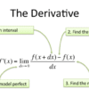
The derivative of a feature f( x) is signified in many ways but frequently utilizing the icon’ called prime as in F( x), review “f prime of x.” The derivative offers the instantaneous price of modifying the dependent variable y as the independent variable x comes close to 0. Let us consider a particular instance to make good sense of this gibberish. Allow us take the function s = -16 t ^ 2 + 60t + 5. If you have read several of my other short articles, you identify this equation as a second-degree polynomial int or a quadratic; because of this, the graph, or image that it produces, is that of a parabola. Furthermore, given that the coefficient of the t ^ two terms is -16, the parabola opens down.
Details on Antiderivative Calculator
In the above function, the independent variable is t and the dependent s, entirely analogous to x and y in various other parts. The reason s and t are utilized here is that this function provides the range an item falls in space based on the planet’s gravitational area and below t stands for time and also s distance. Now the by-product of this feature, s'( t), provides the rapid price of modification of s as the adjustment in succeeding time intervals approaches 0. If we examine the feature as the time comes on the ever-smaller sized intervals-for instance, as time goes from 1 2nd to one nanosecond later-then, we are getting close to what we imply by a rapid rate of modification.
If we take the derivative of this distance feature s, we obtain s'( t) = -32 t + 60. Surprisingly, this ends up being the rate or velocity of the object that the initial function is defining. That’s right. The by-product of the distance feature provides the rate. For instance, at t = 1 second, the original part considers that the distance dropped is 49 feet (where t is in seconds and s remains in feet). You obtain this by plugging one into the original feature. The velocity at this split second is 28 ft/sec.
Swe sometimes, we understand the feature for but ever, not the range, the concern becomes can we locate the for that which defines distance? This is where the antiderivative is available. For example, let us begin with the rate feature, which we will call.
Solving Problem with Antiderivative Calculator
v(t) = -32 t + 60. If you see, this coincides as s'(t) above. Using the process of assimilation or antidifferentiation, we can discover the feature s(t) by discovering the antiderivative of v(t) = -32 t + 60. Making use of strategies we will explore in another series of posts, the antiderivative becomes -16 t ^ 2 + 60t + c, where c means a constant. If you compare this to the initial distance feature, you will see that c must be 5 for them to agree. So why do we get simply c after we take the antiderivative of the velocity function?
The solution is that when we take the derivative of a constant, we get 0. When we antidifferentiation any function, we need always to enable a number to be there, considering that it disappears when we take the by-product. This might appear a little complicated, but this will undoubtedly become more apparent in another collection of posts. Eventually, we need to ask how we return to that original distance feature in which c = 5. The solution is that we utilize something called initial conditions. For example, if we are provided with the speed function and informed that the distance of this particle at time 0 is 5, we can then identify c to be 5.
The derivative and antiderivative are two essential elements of calculus, and also, without a doubt, they create 2 of its bare branches: differential calculus and integral calculus. To adhere to some posts that disclose more concerning the antiderivative’s inner workings and applications. See you after that.
The limit is nothing more significant than a value approached by a function when we let the independent variable become arbitrarily close to some value. Aside from specifying the derivative- a crucial feature in all of the calculus- the limitations enable us to discuss things like division by zero. Exactly how odd!
Final Words
Initially, we looked at the feature y = 1/x and analysed the limit of this function when x approached two and much more surprisingly when x approached 0. The latter examination compelled us to realize what department by absolutely no indicated: that of infinity. To put it simply, department by zero is classified as undefined since we cannot place a set value on infinity. Infinity, by its very nature, is vague. Besides, just how large is infinity? You can think of the magnitude of space, and also, its size still fades in comparison to utmost infinity. Yes, without a doubt. Infinity is a highly unusual idea. (See extra on this in my collection of short articles Dabbling in Infinity).
After checking out the initial write-up, you still may be wondering what is so unobvious concerning this principle of limitation, for in the instance of y = 1/x, except x coming close to 0, any other limitation value can be computed by straight replacement. Hence the limit of this feature when x comes close to 3 is 1/3. If we examine the rational function, the limit when x comes close to 10 is 1/10, and so forth.
Example
Y = (x ^ 2 + 5x + 4)/( x + 4) as well as ask what is the limit of this feature when x comes close to -4, we can not calculate this by direct substitution as the value of the function is undefined right here given that the common denominator becomes zero. What we perform in this case is make use of an algebraic simplification of the good part as well as compose.
( x ^ 2 + 5x + 4)/( x + 4) as (x + 4)( x + 1)/( x + 4). We after that make use of the cancellation building of department to obtain.
( x + 4)( x + 1)/( x + 4) = x + 1 (Canceling the (x +4) from both the numerator and common denominator). Now we can examine what occurs to this algebraically equivalent function at values distinct from -4. For when x is not equal to -4 but obtains completely close to -4, then the limit of the original reasonable feature will come close to x + 1 or -4 + 1 or -3.
More Details on Antiderivative Calculator
Bear in mind. The limit principle does not imply that the independent variable gets to equate to the value concerned. But approach it sufficiently close. This idea, in effect, appears to provide us with a free ride. For example, we cannot split by absolutely any, but we can divide by numbers. That obtain so close to zero that they are as near no as virtually being no themselves. In the example of the rational function just reviewed. Ee cannot discuss the value of the process when x = -4, but we can discuss its value. When x takes on values completely near to -4.
This “free ride” largesse, given to us by the concept of limitation, opens an entire world of higher maths. As well as provides us with the capacity to compute amounts that, without such a great concept. It would certainly be merely enormous. Hence, we move to the derivative via the limit. A unique limitation we will go over in an upcoming write-up and from here to the antiderivative or essential. We can make such points as calculate irregular locations and volumes. Quite a give from such a simple idea!